Preposterous Preponderance

This is a challenge about the collection of far too much, and what to do with it. It involves a lot of combinatorics and algebra.
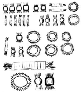
Distribution of Candy and close view of each type.

Halloween! Perhaps it would be better if there wasn’t candy involved. It causes … problems. But alas: you went and got far too much. Now you face the consequences: you need to sort the candy, and of course, there’ll be one kind of candy that is your favourite, and you’ll have none of it. And then there’ll be another kind that you have scores of, but hate. This is when you’ll have a brilliant idea: trade! However, you run into a problem. Each trade benefits both parties, but how to determine if the benefit is equal? Does it matter? When you were less unlucky with candy, or just were too young to worry about this sort of thing, it was easy. But with enough effort, we can make it hard:

  • The value of a candy is inversely proportional to how many of it you already have
  • The optimal value would be achieved by distributing each type of candy equally
  • You have some of more kinds of candy than others, as do your friends—but they have different kinds.
  • You can trade a collection of candy for another by mutual agreement
  • Since you’re so clever, you can make any binding agreement about exchanges of candy.
  • You can waste as much time as you like discussing the sharing of your candy

If the first candy of any type provides a value of 1, determine the value that would currently be achieved, the optimal total value if candy is distributed equally, and the total value that will be achieved by rational exchange, for the following assortment:

CandyAliceBobCarol
A420
B216
C360
D114

Solution to Kayoed Kangaroo

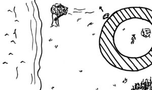
Kangaroo chasing Sheep

Kangaroo was bumped by Sheep. Now Kangaroo is angry, and the chase is on: can Sheep escape? No. Of course not.

Sheep runs 10 meters away in a single second, but Kangaroo is not worried. Kangaroo jumps directly toward Sheep, but is still 1 meter out of range. But no matter where Sheep runs, Kangaroo will jump behind, so that Sheep is just over 6.5 meters away. Sheep is forced to run directly toward the pond.

Perhaps, if Kangaroo were not quite so fast, Sheep could have escaped. Sometime later, perhaps we will discuss a scenario where Kangaroo jumps only thrice per second, and Sheep flees at 9 meters per second.

Kayoed Kangaroo

This challenge considers an upset kangaroo making a series of discrete jumps in order to retaliate, and thus involves trigonometry.

Kangaroo chasing Sheep

Red Kangaroos in Australia compete with sheep for food. Sheep is grazing when it bumps into Kangaroo. The kangaroo wishes to learn the sheep some respect by either pummelling it, or pushing it into a nearby pond. Sheep wants to escape Kangaroo, but is slower than Kangaroo. However, Kangaroo is only capable of moving in jumps. Ergo, if Sheep stays far enough away to avoid pummelling, but too close for Kangaroo to jump, it is safe, and thus can avoid retribution indefinitely. Precisely formulated:

  • Kangaroo can jump up to 8 meters
  • Kangaroo cannot jump fewer than 5 meters
  • Kangaroo can jump at most fource per second
  • Kangaroo can pummel the sheep they are within 1 meter
  • Sheep can flee at 10 meters per second
  • Sheep can flee for 1 second before before Kangaroo pursues
  • There is a nearby pond, a perfect circle and 100 meters in radius
  • Sheep does not like swimming or being pummelled;
  • Kangaroo wishes to punish Sheep for perceived slight

Therefore, the challenge is thus: what is the maximum distance from the pond from which Kangaroo can punish Sheep?

Solution to Curt Cutting

From a deck of n cards, we cut—randomly select with replacement—10 different cards before cutting a card we had seen before. We are trying to determine the probability of achieving this result for n from 10, the lowest n for which result is possible, up to n < 30.

{10\over10}\cdot{9\over10}\cdot{8\over10}\cdot{7\over10}\cdot{6\over10}\cdot{5\over10}\cdot{4\over10}\cdot{3\over10}\cdot{2\over10}\cdot{1\over10} \cdot{10\over10}\ =\ {9!\,10\over10^{10}}\\[16pt] \operatorname P n \propto {(n-1)!\,10\over (n-10)!\,n^{10}}
Probability distribution of n

For n = 10, the calculation is simple and shown above. For n = 11, is the calculation more complex? No: 10!9/1110 works! However… this does not work for n = 12. 11 * 10 … 2 does not match the equation used above to derive the formula. It should be 11 * 10 * … 3, of course. With that error avoided, the formula above is produced, and this can easily produce a probability distribution. The expected value of n is then easily calculated to be ≈23.31.

Curt Cutting

This challenge is about cutting cards. And therefore about probability and combinatorics.

You have a deck of cards. For convenience, we’ll just use A-9 to have a nice round 40 cards. You cut some number of cards. At least one quarter and less than 3/4. That’s a neat 20 possible number of cards. To keep things simple, make them all have a probability of 5%. Now, from this cutting you cut a number of single cards, shuffling in between cuts of course. Formally, that’s random selection with replacement. At some point, you will cut a card that you have seen previously. At this point, you stop. This cuts short the data you receive about the deck of cards; you haven’t seen half of them. Of course, one can always estimate the remaining number of cards. So say you cut 10 cards before a repetition (11 cards total), and that for some reason you cannot visually approximate how many cards are in the deck. The challenge is to determine the expected number of cards in the deck.

The expected number of cards, to put it simply, is the “best” guess for how many cards are in the deck given your information. “Best” means minimizing the average difference between the actual number and your guess.

Solution to Cantankerous Circle

We’re trying to determine the average distance from a random point in a circle to the centre, for various definitions of average. The simplest, the arithmetic mean distance, is ≈ .6667.

\iint_R \ln \operatorname f x\ \delta A

First, the geometric mean. The basic integral required to solve this is above. It’s not a very hard integral, especially for a circle. It’s equal to 2π times the integral from 0 to 1 of x2 ln x. That’s a relatively simple integration by parts, which many already know how to do–but for completion:

\int_0^1 x^2 \ln x\ \delta x \\[16pt] \int_0^1 \ln x \cdot x^2\ \delta x \implies \xcancel{\left[ {x^3\ln x\over 3}\right]}_0^1-\int_0^1 \frac{x^2}3 \delta x \\[16pt] = {\left[\frac{x^3}9\right]}_0^1 = -\frac19

Substituting, the geometric mean distance is e-2/9 ≈ .8007. Note that this is -2/9 not -1/9 because we multiplied the integral by 2π.

Second: the quadratic mean. Since we’re using the identity function, this is a rather easy one. The integral of x2 times x is 1/4 x4, from 0 to 1 that’s just 1/4. We take the square root of 1/8, not 1/4, for the same reason as with the geometric mean. Thus, the quadratic mean distance is ≈ .3536.

Third: the harmonic mean. We saved the best for last: the determinant of the transformation from cartesian to polar coordinates is x. 1/x times x is 1. It’s the easiest integral of all! The harmonic mean distance is .5.

And last, the extra easy cool-down problem, that’s not even really integration at all. This one is fairly obvious: the median distance is ≈ .7071.

Cantankerous Circle

The average distance to the centre of a circle is two thirds the radius. For simplicity, say the radius is 1; the average is simply 2/3. How is this average defined? We will be exploring continuous extrapolations of averages using calculus, geometry, and more.

\int_a^b \operatorname f x \ \delta x \, \div (b-a)

We consider this to be the arithmetic mean value of f from a to b. This can be generalized to more than one dimension. But there are other types of average than the arithmetic mean. Consider the following other types of average, specifically applied to a circle:

\iint_R\ln{\operatorname f x}\ \delta A = \ln\text{GM}\cdot A \\[32pt] \iint_R{(\operatorname f x)}^2\ \delta A = \text{QM}^2\cdot A \\[32pt] \iint_R {1\over\operatorname f x}\ \delta A=\frac A{\text{HM}} \\[32pt] \operatorname f n < \text{median}\ \forall\ n \in R_1, \\[4pt] \operatorname f n > \text{median}\ \forall\ n \in R_2, \\[8pt] \iint_{R_1}\delta A = \iint_{R_2}\delta A,\quad R = R_1 \cup R_2

Since, at the origin, some of these means are discontinuous, ignore the boundary. The challenge is to determine the value of these averages for the distance from the centre.

Solution to Spry Springs

We’re trying to determine the characteristics produced by combining multiple springs together in a row. It seems that all the springs should experience the same horse. When a spring is under some amount of compression, if it is not changing in length, it must be exerting an equal outward horse. To simplify, assume the combined spring is not moving. Obviously, a spring moving about will not change its characteristics–unless it is accelerating. So, when a spring has 5 newtons of horse on its left, it also has 5 newtons on its left, and we consider it to be under 5 newtons of compressive horse. Since one spring’s left is on another’s left; they are in a line. The nominal length is the length when a spring is under no horse. When the combined spring is under no horse, all springs inside are also under no horse, and thus the combined spring has a nominal length equal to the sum of the nominal lengths of the component springs. The spring constants may seem a bit more complex, because the horses remain the same, not the displacements. But really, this just means we summate the inverses. So 1 metre per Newton, plus 50 centimetres per Newton, equals 1.5 metres per Newton.

Spring ConstantsNominal lengths
1.42N/m3m
1.091N/m8m
.6154N/m8m
.25N/m15m

Spry Springs

This is a challenge about springs.

Say we have a few springs. They each have their nominal lengths and their spring constants. We wrap them all around a rail, with sliding spacers in between. In this way we have created a larger spring. We are challenged to find a way to compute the characteristics of this spring–importantly, the spring constant–in a general way. This should be a short, fun activity! But really, it’s actually a surprisingly interesting and challenging task. For a simpler task, try only the first example below. To practice your math after finding a formula, try all of the examples below!

Spring ConstantsNominal Lengths
2N/m, 5N/m2m, 1m
3N/m, 4N/m, 3N/m3m, .5m, 4.5m
1N/m, 2N/m, 8N/m4m, 1m, 3m
.5N/m, 1N/m, 1N/m2m, 3m, 10m

Solution to Macrocephalous Measurement

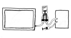
The mechanism measuring the capacity of the large container.

We’re trying to find the volume of the container on the left. First, there is a need to create a system of equations representing the volumes. The linked cylinders will be filled with fluid, to neglect their volume. Let the volume of the measured container be V1, the auxiliary container, V2. Let their pressures be P1 and P2. The atmospheric pressure will be P0. The volume pushed, and remaining volume in the main and auxiliary containers: α, β, and γ respectively. The shift of the cylinder is Δ(γ). Using the fact that pressure times volume is constant for constant temperature, we end up with the following system of equations:

V_1 \cdot P_1 = \alpha \cdot P_0 \\[8pt] V_2 \cdot P_2 = \beta \cdot P_0 \\[8pt] P_1 + P_2 = 2 P_0 \\[8pt] \operatorname \Delta \gamma = \gamma + \alpha – V_1 = \beta – V_2

We know that Δ(50mL) = 30mL in the case given, but for a full solution, a general formula will be given here. But in the general case, the known variables are γ and Δ(γ). The third equation provides the first step: divide both sides of it by P0. This is because the value of atmospheric pressure is not relevant, only the ratios to it! We also divide the first and second equations by P0 to complete the switch, removing the irrelevant variable to enable completion of the problem. You may ask why this variable was included in the solution: for completeness; to demonstrate that it’s unimportant. Next: split the fourth equation as shown below. This easily resolves, separating the volumes from the variables. Note that V1 = α + Δ(γ) – γ, so removing it at present is no problem–it can easily be found later.

\alpha = V_1\cdot{P_1 \over P_0} = V_1+\operatorname\Delta\gamma-\gamma \\[8pt] \beta = V_2\cdot{P_2 \over P_0} = V_2+\operatorname\Delta\gamma \phantom{-\gamma}\\[16pt] \alpha-\alpha\cdot{P_1 \over P_0}+\operatorname\Delta\gamma = \gamma \\[8pt] \beta -\beta \cdot{P_2 \over P_0}\phantom{+\operatorname\Delta\gamma} = \gamma

Combining the last two equations, it becomes easy to find the one in terms of the other. The equation below describes the simplified relationship without knowing the volume of the auxiliary container. Know that V2 = β + Δ(γ), and as we know that V2 = .5L, so β = .5L – Δ(γ). To solve for this specific case–for to only solve generally and not in the specific case would be just as incomplete as would the opposite–we then fill in our known values of Δ(γ) = 30mL, γ = 50mL, and extending to β = 470mL. We get the value of α = (470mL/30mL – 2)(20mL) ≈ 27.33mL. Remembering from before that V1 = α + Δ(γ) – γ: V1 = ≈27.33mL – 20mL ≈ 7.333mL. The answer is then ≈7.333mL for the specific case and the equation below for the general case.

\alpha = \left(\frac\beta{\operatorname\Delta\gamma}-2\right)\cdot \left(\gamma-\operatorname\Delta\gamma\right)